
Somewhere in Denmark, a project manager tasked with Digitalisation in a utility company gets a phone call. The call comes from IT. We all know what that means: trouble. The project manager takes a deep breath and throws himself into the lion’s cage.
PM: Yes?
IT: Are you aware of the amount of data you’re logging into the database?
PM: Yes.
IT: It’s overwhelming the database. Is this all the data you’re logging?
PM: No, that’s less than 10%.
IT: [silence]
PM: [silence]
IT: … that’s not going to work.
And thus, a new journey began to handle large amounts of (time-series) data more efficiently.
Background
Managing massive amounts of time-series data is no small feat, especially for utility companies like our client, a respected player in the water and wastewater sector. When faced with the challenge of efficiently handling their growing data needs, the client turned to us to find a solution.
This case study explores how we leveraged Postgres and TimescaleDB to meet their demands, the reasoning behind our choices, and the lessons learned along the way.
The problems
There are two types of problems they faced:
1. Choosing a scalable solution
The client initially relied on MSSQL to manage their data. However, as their data grew exponentially, it became clear that MSSQL wasn’t scaling well enough to meet their requirements. With hundreds of thousands of data tags and a need for frequent data logging, the system was under significant strain, leading to performance issues and inefficiencies.
2. Deciding what data to use and how often
At the beginning, there was one principle: “let’s just log all tags every 5 seconds”. Six months later, the IT people were quite concerned. The client was already using 7 TB of space… out of the 100-150 TB of space they were likely going to need for 150.000+ tags.
Safe to say, things needed to change.
The solutions
1. The database choice: PostgreSQL and TimescaleDB
Why?
- Free and Open Source: TimescaleDB is built on Postgres, an open-source relational database system. This made it an attractive option for the client, offering flexibility without additional licensing costs.
- High Compression Ratios: TimescaleDB’s native compression feature allows us to store large amounts of data efficiently. For example, 100 GB of raw data can be compressed to just 10 GB, significantly reducing storage requirements and system load.
- Built for Time-Series Data: TimescaleDB is specifically designed to handle time-series data. It supports hypertables, which allow partitioning of time-series data while maintaining high query performance.
- Continuous Aggregates: This feature enables the creation of continuous aggregate views that automatically update as new data comes in. This is crucial for the client, as it allows them to maintain real-time summaries without constantly recalculating large datasets.
- Easy Integration with Postgres: The ability to use TimescaleDB alongside regular Postgres tables provides flexibility. We can configure the database to store time-series data in hypertables while keeping other relational data in standard tables.
Postgres and TimescaleDB will run in parallel to the existing MSSQL database for 3 months to test performance and minimise risk.
2. Smarter data handling
A crucial step was to analyse the client’s data requirements. This involved understanding what data needed to be stored, how frequently it should be logged, and the specific use cases for the data. We quickly realised that not all data needed to be logged at high frequencies. For instance, filling up water tanks takes a long time—logging water tank levels every five seconds was unnecessary; logging on change or every 20 seconds was enough.
We then restructured the data storage approach:
Splitting data into multiple databases
Instead of a single, overloaded database, we divided data into multiple databases based on types of data points. For example, commands, states and setpoints were stored in a table in one database and measurement values were stored in a table in another database.
The data was split up into 4 different databases:
- Setpoints, states, commands
- Counters – number of starts of a motor
- Accumulated values – This could be power usage over an hour or the amount of rain in the current hour or day
- State values – temperatures, voltage, RPMs, level in a tank etc.
The reasoning behind splitting up the data like this is twofold:
1.The data is split up into smaller chunks, which makes for faster queries.
2. The aggregations are different for each database. If everything was in the same database, we would have another problem: for every 5-mins or 1-hour aggregation, it would’ve had to first filter out the different data points and decide which type of aggregation should be done. Splitting up the data upfront solved that headache without any effort:
- Setpoints, states, commands – No aggregations;
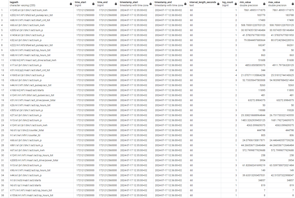
- Counters – Min, Max
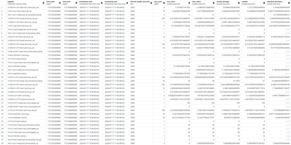
- Accumulated values – Min, Max, Average, Median and standard deviation
- State values – Min, Max, Average, Median and standard deviation.
This separation eased the load on each database and made querying more efficient, but it also made analysis easier—you know what type of data you’re dealing with and what type of analysis you can make without having to think about it too much.
Adjusting logging intervals
We set different logging intervals for different types of data. For example, some critical data points were logged every second, while others, like water level changes, were logged less frequently. This reduced unnecessary data logging and optimized storage usage.
Implementing continuous aggregates
We defined continuous aggregate policies for different datasets. For instance, the client needed hourly averages of certain data points. By setting up these aggregates, we ensured that the data was pre-processed and ready for analysis, reducing the need for on-the-fly calculations.

Challenges and Lessons Learned
Transitioning to TimescaleDB wasn’t without its challenges. Here are some key takeaways:
- Initial data overload: Early on, the client wanted to log all data at very high frequencies. This quickly filled up the database, highlighting the importance of being selective and intentional about what data to log and how often.
- Maintenance overhead: While splitting data into multiple databases improved performance, it also increased maintenance complexity. Managing several databases requires diligent oversight and regular maintenance.
- Scalability concerns: The continuous aggregate and compression features were pivotal in choosing TimescaleDB. However, scalability remains a critical consideration. It’s essential to continuously monitor performance and adjust configurations as needed.
- Balancing act: Finding the right balance between too much and too little data logging is crucial. Over-logging can bog down the system, while under-logging might miss critical data points. It’s a learning process to find the sweet spot.
Conclusion
This solution is still in the testing phase. While there are still lessons to be learned and adjustments to be made, the client is now one step closer to handling their data needs more efficiently, ensuring they can continue to provide reliable services in the water and wastewater sector.